
Introduction
Over the last several months, we showed how to use near-field probes to characterize and interpret dominant harmonic energy sources on PC boards and how to use RF current probes to characterize the coupling of these energy sources to power and I/O cables. This time, we’ll discuss how to use a nearby antenna to monitor actual emissions from a product or system.
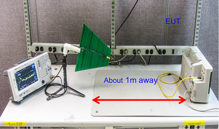
While many designers attempt to perform radiated emissions troubleshooting at an outdoor site or in a semi-anechoic chamber using a third-party test lab facility, I’ve found a much more efficient method is to perform this using a nearby antenna right on your own work bench (Figure 1). Performing this testing in-house also allows additional tools and resources to be close at hand.
Best of all, a calibrated EMI antenna is not really required, as all we care about are relative changes! In one case, I was testing an industrial printer and connected a 1m-long piece of wire to the spectrum analyzer and stretched it out nearby. I’ve even had clients use a nearby Wi-Fi antenna for troubleshooting. So long as you can see the harmonic emissions, you can try various mitigations and observe the results in real time!
Some may question the use of an antenna so close to the product under test, as this is within the near field at the lower frequencies. While near field measurements can’t be directly compared to far field measurements, for troubleshooting purposes we’re just looking for relative changes, not absolute. For example, if we know we’re failing at 230 MHz by 5 dB, then we’ll strive to lower that on the work bench by 10 dB or more, just to be safe.
If you wish to compare with actual compliance test lab data, you’ll need to space a calibrated antenna at 3m or 10m and account for all the measurement system losses and gains. We’ll describe how to do that next time.
Currently, the antenna I prefer is a log-periodic design built from PC board material. These are available at low cost from Kent Electronics (http://www.wa5vjb.com), and the larger 400 to 1000 MHz model I prefer costs just $53 (with attached SMA connector) as of this writing. While not resonant in the range 30 to 400 MHz where most of the larger harmonic emissions reside, I’ve found that positioning the antenna about 1m from the EUT allows me to see the emissions well enough to troubleshoot.
I published an article a few years ago that describes how to make the PVC fittings to hold the antenna and fasten it to a simple table-top camera tripod (Reference 1).
Troubleshooting Process
By now, you should have characterized the emissions profile of the dominant harmonic energy sources within your product using near field probes, as well as characterized the couplings to interior and exterior cables using an RF current probe.
With this data in mind, it should be easier to identify the specific sources and couplings that result in radiated emissions. The usual “radiating structures” will include I/O and power cables and seams and apertures in shielded products. For the majority of unshielded products, it will be cable or PC board radiation (or both).
Most narrowband emissions will tend to be grouped around 50 to 300 MHz and are largely due to radiating structures that start to approach 1/4 to 1/2 wavelength. For example, a 1m long cable (typical USB) will resonate at 45 to 100 MHz, depending on whether the shield connects to PC board or line-powered product with a shielded chassis. Refer to my article on cable resonance in Reference 2.
Ambient Transmissions
One problem you’ll run into immediately when testing radiated emissions outside a shielded room is the number of ambient signals from sources like FM and TV broadcast transmitters, cellular telephone, and two-way radio. This is especially an issue when using external antennas.
I’ll usually run a baseline plot on the analyzer using “Max Hold” mode for a couple of minutes to build up a composite ambient plot. Then, I’ll activate additional traces for the actual measurements. For example, I often have at least two plots or traces on the screen: the ambient baseline and the actual measurement. It greatly helps to become familiar with your area’s RF spectrum usage.
Fortunately, there are three ways around this:
- In most cases, you’ll observe a range of product emissions in a harmonic relationship. Very often, these harmonics are created from the same source, and if one or more are masked by ambient signals, then working on the others that are more visible will generally bring the whole batch down, as well.
- In some cases, there will be a critical harmonic masked by an ambient transmitter. A common example is a 100 MHz harmonic hidden underneath a strong FM broadcast station at the 99.9 MHz channel. In this case, I’ll try reducing the resolution bandwidth from 100 or 120 kHz down to as little as 1 kHz or less. This often “filters out” the modulation from the FM station, allowing you to observe the hidden harmonic. This also presumes the harmonic is an unmodulated continuous wave (CW) signal. Just be sure reducing the RBW doesn’t also reduce the harmonic amplitude. If your harmonic is modulated, this may not work, so you could try selecting a higher related harmonic, as in (1) above.
- Move your testing well away from urban transmitters (easier said than done these days) or test in the early morning hours.
Remember that strong nearby transmitters can affect the amplitude accuracy of the measured signals as well as create mixing products that appear to be harmonics, but are really combinations of the transmitter frequency and mixer circuit in the analyzer. You may need to use an external bandpass filter at the desired harmonic frequency to reduce the effect of the external transmitter. An example would be an FM broadcast band “stop band” filter.
Mitigating Couplings Paths
Now that we can observe the actual emissions from the EUT, we need to turn our attention to the coupling paths that connect the internal energy sources to radiating structures. In the near field environment of a typical table top product, we’ll most likely be dealing with capacitive and inductive coupling.
Capacitive coupling is mainly due to large changing voltages with time (high dV/dt) and can be modeled as two plates near each other. A good example is the fast-changing switching voltage of a typical DC-DC converter. The coupling could be occurring between the switch device’s heat sink and a nearby ribbon or flex cable.
Inductive coupling is mainly due to large changing currents with time (high di/dt) and can be modeled as two loops near each other. Cable-to-cable coupling is a good example. Another example would be cable-to-transformer coupling.
If clock harmonics are being coupled to cables and radiating, then you’ll need to look at your PC board layout and stack-up. Are clock traces running too close to I/O traces? Is the clock oscillator or resonator located too close to an I/O connector?
When it comes to internal PC board couplings I find it’s often due to a poor choice in stack-up design. For best EMC performance, every signal layer should have an adjacent solid return plane. As well, every power plane or routed power layer should also have an adjacent solid return plane. For more information, refer to my series on low-EMI PC board design with part 1 starting in Reference 3.
System-level issues can also lead to radiated emissions. For example, how internal cables are routed can make a big difference. Is there an internal flex cable routed too close to one of your high-energy sources? Are motor drive cables routed in the same bundle as sensor or I/O cables? Known noisy cables should always be separated from quiet signal or I/O cables. A really good troubleshooting technique is to remove I/O cables one by one while monitoring with the antenna.
For shielded products, all sheet metal must be bonded together at frequent intervals. Long seams between enclosure pieces can act as radiating antennas if the length starts approaching 1/4 to 1/2 wavelength. Ott (Reference 4) has a chart of shielding effectiveness versus slot length versus frequency. For example, a slot length of 2 inches (5cm) has a shielding effectiveness of only 10 dB at 1000 MHz. A good design goal would be a shielding effectiveness of 20 dB, which would require seam lengths of just 1/2-inch (about 13mm) at 1000 MHz. Keep this in mind for ventilation patterns.
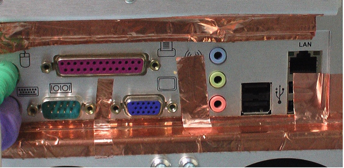
Adhesive copper tape is a good troubleshooting tool when applied over possible seams (Figure 2). A near field probe (either H- or E-field) can help identify longer seams. I typically use a marking pen to identify the beginning and end of a leaky seam. Then, I can measure the length and use that with the dominant frequency to assess whether the seam is approaching resonance.
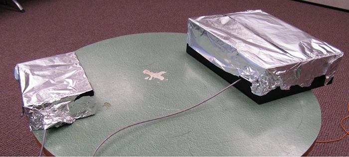
For products with metal enclosures, apertures, like LCD displays, keyboards, and ventilation holes can also be sources of emissions. A common issue with LCD displays is the lack of bonding between the display housing and product enclosure. Using copper tape or EMI gasketing are good mitigating techniques. It’s not unusual for me to cover an entire product with heavy-duty aluminum foil during troubleshooting while I carefully cut out around potential apertures one at a time in order to identify the dominant emission source (Figure 3).
Summary
The last several installments of EMC Bench Notes have covered my basic approach to troubleshooting one of the most common EMC issues, that is, radiated emissions. My process of characterizing energy sources with near field probes and then measuring cable harmonic currents with a current probe and following up with a close-spaced antenna has proven to be a fast and efficient way to attack emissions over several decades. I’m sure it will help you as well.
Next month, we’ll explore how to set up an in-house or temporary pre-compliance setup for measuring absolute levels of radiated emissions where you can compare to official test limits. While there are obvious issues when testing outside a shielded semi-anechoic chamber, this method will help confirm pass/fail well in advance of final compliance testing.
References
- Wyatt, “PC Board Log-Periodic Antennas,” EDN, https://www.edn.com/pc-board-log-periodic-antennas/
- Wyatt, “Measuring Resonance in Cables,” EDN, https://www.edn.com/measuring-resonance-in-cables/
- Wyatt, “Design PCBs for EMI, Part 1: How Signals Move,” EDN, https://www.edn.com/design-pcbs-for-emi-part-1-how-signals-move/
- Ott, Electromagnetic Compatibility Engineering, Wiley, 2009, Figure 6-27.