
Control of low audio frequency magnetic fields from cables, as required by some spacecraft EMI control standards, is best implemented as a conducted emission measurement, but these may require exceptionally efficient transducers and techniques, which are discussed herein.
Common-mode conducted emission (CMCE) limits and measurements are often specified within spacecraft EMI standards, such as the Space & Missile Command’s SMC-S-008, EMC Requirements for Space Equipment and Systems [1], and the NASA Goddard Space Flight Center’s General Environmental Verification Standard (GEVS) [2].
Above audio frequencies, the rationale for such control is generally either the control of cable-to-cable crosstalk, and/or indirect control of radiated emissions. Such control and measurement is much more accurate and repeatable than radiated measurements when the cable is electrically short.
At audio frequencies, effective cable design usually precludes interference from crosstalk. There is no need to control CMCE at audio frequencies unless an unusually low-level signal is carried by a cable, and/or there are restrictions on the quality of shielding available, or the ability to twist a signal with its return.
But there is a special case where the control of CMCE at frequencies down to the very low end of the audio spectrum is desirable, and that is when a platform has a magnetic cleanliness requirement. Such platforms carry sensitive magnetometers. A sample derivation of such a limit is presented.
Background
Consider the variable-mu magnetometer pictured in Figure 1. While this is earthbound test equipment, it will be shown that its sensitivity corresponds well with existing CMCE requirements in references [1] and [2].
The EMCO 6640 has 50 kHz bandwidth and 60 dep’t wideband sensitivity. An EMI receiver connected to its analog output can tune in narrowband signals down to 13 dBpT (13 dBpT + 10 * log (50 kHz) = 60 dBpT).
An EMCO 6640 or similar device can measure the field from a test sample and its interconnecting cables by specifying a distance and configuration of the test set-up and sensor. In fact, this has been done in the 1967 vintage RE04 MIL-STD-461 requirement and MIL-STD-462 test method.
Such a control may be valuable for an equipment housing, but since such fields fall off with the cube of distance (at distances where the equipment dimensions are small relative to the separation distance), it is most likely cables will be the culprits. Also, an optimally designed platform will separate magnetic sensors from localized magnetic hotspots, but it may be more difficult to separate sensors from any and all cables. Finally, magnetic emissions from cables fall off directly with distance (or in the case of cables above a conductive ground plane, as the square of distance) so that cable CMCE, although nowhere near as “hot” as a motor or transformer, may appear so at a distance.
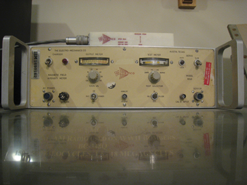
Figure 1: Electro-Mechanics Company EMCO 6640 variable-mu magnetometer (circa 1964).
In order to derive a CMCE limit from a magnetic flux density limit such as 13 dBpT, it is helpful to convert from units of flux density to magnetic field, assuming free space permeability.
The basic relation B = μH converts to dBpT = dBuA/m + 2 dB uH/m in log-space. Hence, 13 dBpT is 11 dBuA/m.
If a cable far from ground carries a current “I” causing a circulating magnetic field “H”, that relationship is the familiar H = I/2πr.
Assuming a separation of one meter between cable and sensor and converting to log-space, an H-field of 11 dBuA/m implies a common mode current on the cable of 27 dBuA. However, the more common situation is that the cable is near a conductive ground plane, and if the height above ground “s” is small relative to the observation distance “r”, then the relationship between the common mode current and resultant circulating magnetic field is H = I (2s)/2πr2
For a typical case where “s” is 5 cm and “r” is 1 meter, the above equation introduces a 20 dB relaxation in the allowable cm current, which is then 47 dBuA rather than 27 dBuA.
The ground plane is our friend! Compare this computed value of 47 dBuA with the Figure 2 CMCE low frequency plateau limit in the two standards cited in the Introduction.

Figure 2: Existing spacecraft CMCE limits.
The previous derivation does not prove that the low frequency CMCE limits shown in Figure 2 are derived from magnetic cleanliness requirements; the actual origin of the GEVS limit is shrouded in the mists of time. The derivation only goes to show that such a CMCE limit can be very useful in controlling magnetic cleanliness. The SMC limit is a GEVS derivative: it has no separate lineage. It differs from the GEVS limit in that it applies to the total CMCE from a unit, as opposed to just the power interface or individual cables. The SMC limit is measured by lifting the unit off ground, reattaching it via a wire, and measuring the CMCE through that wire, or alternatively by clamping a current probe around all the cables emanating from the unit.
As this is written (late 2011), the existing GEVS CMCE requirement applies only to power lines. However, a revision currently in process will extend applicability to all cables. The new revision will also relegate the requirement below 150 kHz to those platforms with a specific need for magnetic cleanliness, with the generally applicable limit above 150 kHz being based on crosstalk control. The 30 Hz to 50 MHz SMC limit applies to all platforms and all cables, with possible extensions to both lower and higher frequencies on a platform-dependent basis.
Finally, before moving on to CMCE test methods, it should be noted that another common form of such control is through design requirements mandating balanced above-ground circuits, or single-ended circuits, with dc isolation between signal returns and ground. This is practical at audio frequencies where uncontrolled parasitics will not perturb basic circuit functions.
Test Equipment – Current Probes
A preferred technique for making audio frequency CMCE measurements is the legacy current probe-based CE02 measurement of MIL-STD-462 (1967). However, current probes available in most EMI test facilities (Figure 3) are not efficient enough to measure accurately at a level 6 dB below 50 dBuA (the Honeywell 3892 being a possible candidate, but are long obsolescent and only available if the test facility already owns one). To assess how efficient a transducer must be, the noise floor of the EMI receiver or spectrum analyzer must be known. Published specifications for the Rohde & Schwarz EMI receivers and spectrum analyzers show a noise floor at 30 Hz above 20 dBuV. Obsolescent machines such as the HP8566, designed to be used above 100 Hz but often “pushed” down to 30 Hz with resultant degraded noise floor, show even higher noise levels at 30 Hz (Figure 4). If the goal is to accurately measure a 30 Hz signal at 50 dBuA with a noise floor at 20 dBuV, the current probe transfer impedance cannot be less than -24 dB Ohm. None of the current probe transfer impedances in Figure 3 are adequate for that task.
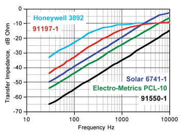
Figure 3: Transfer impedances of typical EMI current probes employed in the CE01/101 frequency range.
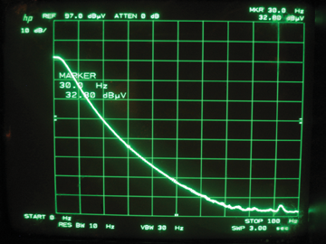
Figure 4: Degraded noise floor of HP 8566B spectrum analyzer below 100 Hz: about 33 dBuV at 30 Hz.
Traditional EMI test current probes are based on ferrite cores. Cores constructed of other available materials, similar to laminated transformer cores, have better low frequency response. Transfer impedances of three such commercially available low frequency probes are shown in Figure 5.
![]()
Figure 5: Transfer impedances of three Pearson Electronics wideband current probes. (Note: These probes are designed with 50 Ohm output impedances, and the plotted curves were made with a 50 Ohm network analyzer. If driving a 1 Megohm oscilloscope input, the plateau is 6 dB higher than shown. Thus, the Model 4688 is time domain spec’d as a 1 V/A probe with a lower 3 dB frequency of 600 Hz, the Model 5101 is spec’d as a 0.5 V/A probe with a lower 3 dB point at 150 Hz, and the Model 3525 is spec’d at 0.1 V/A, with a lower 3 dB point of 6 Hz. Source: the Pearson Electronics web site at http://pearsonelectronics.com.
Comparison of Figures 3 and 5 reveals that the least efficient Pearson probe is about 20 dB more efficient than any of the Figure 4 probes except the obsolescent and very scarce Honeywell probe. Additionally, all the Pearson probes are more efficient than the Honeywell model below 60 Hz.
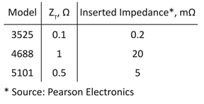
A current probe inserts impedance into the line around which it is clamped. Generally, the inserted impedance is the transfer impedance divided by the turns ratio. For the special case when a resistor shunts the probe output, the inserted impedance is the shunt resistance divided by the square of the turns ratio. For the three Pearson probes discussed herein, the inserted impedances are negligible:
Test Equipment – Current Probe Alternative
For measurements on power lines or between a unit case and ground, the transformer method pioneered by the Solar Electronics Company can be adapted to provide even more efficient low-level, low frequency measurements. If measurements on individual cable bundles are necessary, an efficient current probe such as those discussed previously, is necessary. Regardless, the transformer method may still be helpful under certain conditions.
The transformer method is based on Solar Application Note AN62201, which has been around long enough that it was adopted by the United States Army and included in the 1971 Notice 3 to MIL-STD-462 (the “pink notice”). The application note, found in any edition of the Solar Electronics Catalog relies on the fact that a current probe is a type of transformer; therefore, a different kind of transformer may be substituted. The connection into the circuit, shown in Figure 6, is the same as for MIL-STD-461 CS01 or CS101. But instead of driving the Model 6220-1 coupling transformer with a power amplifier, the transformer’s primary side is connected to an EMI receiver or spectrum analyzer. A loading resistor shunts the primary side to reflect a resistance into the secondary. The resulting transfer impedance has a flat asymptotic plateau at frequencies where the transformer’s reactance is higher than the shunt resistance.

Figure 6: The Solar 6220-1 audio frequency coupling transformer used as a current probe (Source: Solar Electronics catalog application note).
The principle of operation is that the secondary, unloaded on the primary side, has about 1.2 mH inductance. The reactance of that inductance, shunted by different resistors, yields a family of curves as shown in Figure 7. Because of the Model 6220-1 turns ratio of 2:1 primary to secondary, the transfer impedance plateaus in Figure 7 are equal to one-half the shunt resistor value in the circuit of Figure 6. [3] Given the 1.2 milliohm secondary inductance, the highest transfer impedance available at 30 Hz is about -13 dB Ohm. That value is obtained with no load, which is inadvisable since that would insert the entire 1.2 mH inductance into the power-line impedance. That is known to cause switched mode power supply instability. [4] The problem can be avoided using a 1 Ohm shunt, reflecting 0.25 Ohm into the power-line. Transfer impedance degrades 1 dB to -14 dB Ohm, which is the maximum practical transfer impedance available with this technique. This is 8 – 12 dB better than the various Pearson probes achieve.
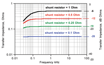
Figure 7: Solar 6220-1 transfer impedance using various shunt resistors on the primary side.
If even better low frequency sensitivity is needed, say if the custodians of SMC-S-008 extend their CMCE limit below 30 Hz, an ordinary 50 or 60 Hz power transformer can be of assistance. A 60 Hz 120 V transformer primary stepping down to 25.2 volts and 2 amp load current yielded the transfer impedance shown in Figure 8, when the primary was loaded by 10 Ohms and the secondary was used to carry the current. A large increase in sensitivity is attained, acquired at the cost of inserting almost 0.5 Ohms in series with the circuit-under-test. Of course, the possibilities here are only limited by access to the power transformer of choice. It should be noted that somewhere between 1 to 10 kHz the power transformer performance deteriorated, and at 1 Hz the measured current waveform was distorted. A 50 Hz transformer could be expected to work to a slightly lower frequency, and the upper limit issue is not a problem because the 6220-1 or a current probe with adequate sensitivity is available at and above 1 kHz.

Figure 8: Transfer impedance of a step-down 60 Hz power transformer with primary shunted by 10 Ohms
Common Mode Measurements
In addition to efficient transducer factors, a key property of a current probe to be used for making pure differential or pure common mode measurements (measurements that involve multiple conductors passing through its window) is adequate rejection of the undesired mode. The Pearson probes all provide at least 80 dB of differential mode rejection when used to measure common mode current up to 10 kHz. Brand new models 4688 and 5101 measured upwards of 90 dB rejection, but EMC Compliance’s well-used Model 3525 measured just over 80 dB. The cases are identical in construction, so hard use accounts for the difference. Figure 9 is a plot of traditional CE01 limits superimposed on the CMCE limit of Figure 2. The dm rejection of the cm test method must exceed the difference between the CE01 limits and the CECM limits. The 80+ dB rejection of the Pearson probes more than suffices, except for the most relaxed GEVS CE01 limit. In the new GEVS, that limit is replaced by MIL-STD-461F CE101, with a low frequency plateau of 100 dBuA. For such a standard, the cited probes are a solution to making these sensitive cm measurements.
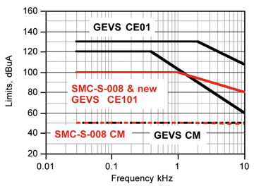
Figure 9: CE01 and CECM limits for GEVS and SMC-S-008
To achieve maximum rejection of the undesired mode with multiple wires penetrating the window, it is necessary that the wires be tightly coupled to each other and centered in the window, so that capacitive coupling between either wire and the grounded current probe case is nearly equal. This is normally achieved with a split nonconductive dowel drilled down the center to take the two wires. It must be long enough so that wires clearing it drape away from the current probe body, and its diameter is just less than the probe window.
Using a pair of Solar 6220-1s to implement the transformer method in lieu of current probes, Figure 10 transforms into Figures 11 through 13. An important difference between hinged current probes and transformers is that a current probe may be opened and closed and wires rearranged within it without disturbing the flow of current to the test sample. The same is not true for a transformer. However, because the primary side is isolated from the current carrying secondary, the sense in which the primaries are connected to each other can be changed without disturbing the flow of current to the test sample, which is a blessing for any device which has to “boot” and requires significant time to reach proper operation subsequent to power cycling. The only difference between Figures 12 (cm measurement) and 13 (dm measurement) is how the bnc-to-banana adapters interconnect. Connections to the secondaries, shown in Figure 10, don’t change.

Figure 10: CM measurement on left; dm measurement on right.
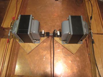
Figure 11: CM/DM measurements made using a pair of Solar 6220-1 coupling transformers. The connection of the primaries (expanded on in Figures 12 and 13) determines which mode is measured and which rejected.

Figure 12: CM measurement connection close-up. The EMI receiver connection shown in Figure 10 has been removed for clarity.
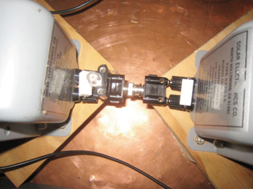
Figure 13: DM measurement connection close-up. The EMI receiver connection shown in Figure 10 is there, but the connecting coaxial cable has been removed for clarity.
For optimal rejection of the undesired mode, it is critical that the two transformers have exactly identical transfer impedances. Of course, this criterion is unachievable in practice, and although this technique produces more efficiency than the use of a current probe, the use of a single current probe to reject the undesired mode will always be superior. Undesired mode rejection is enhanced by using shunt resistors of lower resistance than the reactance of the transformers at the desired frequency. In this investigation, each transformer was shunted by 0.47 Ohms, for a net shunt resistance of about 0.235 Ohms. That compares favorably with the reactance of 1.2 mH at 30 Hz being 0.22 Ohms. Nevertheless, the maximum undesired mode rejection was about 40 dB.
Inspection of Figure 9 reveals that 40 dB differential mode rejection is insufficient to yield accurate cm measurements, because the dm limit is much more than 40 dB above the cm limit. However, the vast majority of electronic loads do not generate noise below the dc-dc converter frequency, and in that case the 40 dB value will be perfectly adequate. Low audio frequency conducted emissions are usually generated by rotating machinery of one kind or another, so if the test sample performs that sort of function, a current probe is a must.
There is a way around a low dm rejection ratio. This involves a modification to the cm measurement as per SMC-S-008, which requires measurement of total cm current, measured between test sample case and ground by raising the test sample case above ground and connecting it to ground with a wire, as shown in Figure 14.

Figure 14: Total CMCE measurement per SMC-S-2008. The LISN represents a test sample whose metal case is raised above ground and then connected to ground via a wire.
The modification is to replace the current probe with the 6220-1 as per Figure 6, but instead of inserting a power wire, its secondary is inserted in series with the ground wire, effectively making the coupling transformer secondary as shunted by the primary, a series element in the ground connection (in Figure 15).
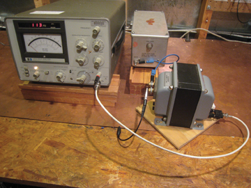
Figure 15: Total CMCE measurement per SMC-S-2008, but using the CS01 coupling transformer in lieu of a current probe.
This technique measures only the common mode current driven into ground, and thus there is no need to reject the undesired mode. It is ideal for working to SMC-S-008, but it is overkill if working to GEVS or any similar requirement that controls CMCE on a per-cable basis. Nevertheless, in the case of the unit that doesn’t generate frequencies below that of its electronic switching power supply, there won’t be any significant CMCE. A total summation of nothing is still nothing.
Conclusion
For the test facility that finds itself rarely working to one of these spacecraft EMI requirements, if the requirement is to only test the power interface, or if an SMC-like total CMCE measurement is made and the test sample generates no noise at audio frequencies, the CS01 coupling transformer technique is a handy way to measure with existing assets and adequate sensitivity. If a test facility is going to be making such measurements routinely, or if the test sample has cable connections beyond power that require individual sampling and generates significant audio frequencies, then the Pearson probes or probes with similar performance are preferable. ![]()
Acknowledgment
Mark Nave’s detailed review of the work contributed greatly to the overall effort and is deeply appreciated. The author would like to thank Pearson Electronics for the loan of Models 4688 and 5101 current probes in developing this article.
References/Notes
- SMC-S-008, EMC Requirements For Space Equipment And Systems, 13 June 2008.
- Goddard Space Flight Center, General Environmental Verification Specification for STS & ELV Payloads, Subsystems, and Components, Rev.A, June 1996.
- This can be understood by recognizing that the resistance shunting the primary reflects across the windings by the square of the turns ratio. That reflected value, multiplied by the current flowing
- through it is converted on the primary side by the turns ratio, so the end result is that the effective shunted value is the primary resistance divided by the turns ratio.
- Javor, Ken, EMC Archaeology: Uncovering a Lost Audio Frequency Injection Technique, In Compliance Magazine, April 2011.
Ken Javor
has worked in the EMC industry for thirty years. He is a consultant to government and industry, runs a pre-compliance EMI test facility, and curates the Museum of EMC Antiquities, a collection of radios and instruments that were important in the development of the discipline, as well as a library of important documentation. Mr. Javor is an industry representative to the Tri-Service Working Groups that write MIL-STD-464 and MIL-STD-461. He has published numerous papers and is the author of a handbook on EMI requirements and test methods. Mr. Javor can be contacted at ken.javor@emccompliance.com.