
This article discusses the creation of a common-mode current in a typical circuit and explains the effectiveness of a common-mode choke on differential-mode and common-mode currents.
Common-Mode Current Circuit Model
Consider a typical circuit model shown in Figure 1.
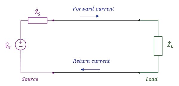
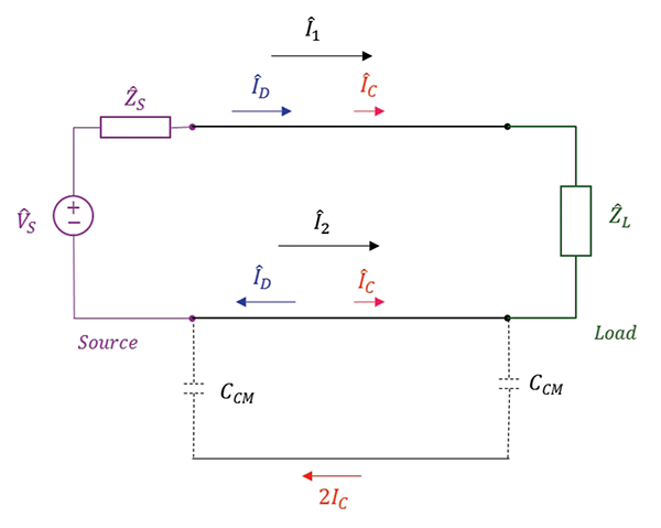
If the fields generated by the forward current cancel the fields of the return currents and no other circuits, or sources, or coupling paths are present, then the forward current equals the return current. In virtually any practical circuit a different scenario takes place, as shown in Figure 2.
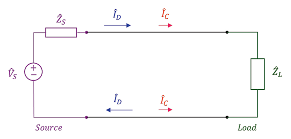
![]() D is referred to as the differential-mode (DM) current while
D is referred to as the differential-mode (DM) current while ![]() C is referred to as the common-mode (CM) current. The DM currents are usually the functional currents, they are equal in magnitude and of opposite directions. The CM (unwanted) currents are equal in magnitude and of the same direction. (In the next section we will show an example of a circuit in which common-mode currents are created).
C is referred to as the common-mode (CM) current. The DM currents are usually the functional currents, they are equal in magnitude and of opposite directions. The CM (unwanted) currents are equal in magnitude and of the same direction. (In the next section we will show an example of a circuit in which common-mode currents are created).
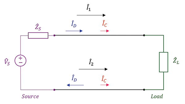
In the analysis of the DM and CM currents we often use the circuit model shown in Figure 3, where, in addition to the DM and CM currents, we show the total currents ![]() 1 and
1 and ![]() 2 flowing in the same direction. The reason for this is that it is easier to apply the classical circuit theory to the total currents than it is to the individual currents. Once the equations are developed for the total currents, we simply substitute the differential and/or common mode currents for the total currents in the derived expressions. This approach will be demonstrated later in this article when discussing a common-mode choke.
2 flowing in the same direction. The reason for this is that it is easier to apply the classical circuit theory to the total currents than it is to the individual currents. Once the equations are developed for the total currents, we simply substitute the differential and/or common mode currents for the total currents in the derived expressions. This approach will be demonstrated later in this article when discussing a common-mode choke.
The total currents ![]() 1 and
1 and ![]() 2 flowing are related to the DM and CM currents by
2 flowing are related to the DM and CM currents by
![]() (1a)
(1a)
![]() (1b)
(1b)
Adding and subtracting Eqs. (1a) and (1b) gives
![]() (2a)
(2a)
![]() (2b)
(2b)
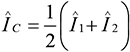
Thus, in terms of the total currents, the DM and CM currents can be expressed as
 (3a)
(3a)
 (3b)
(3b)
Returning to Figure 3 we note that something is missing, since the Kirchhoff’s Current Law (KCL) seems to be violated. Current into the node A is not equal to the current out of the node A:
![]() (4)
(4)
What happened to the total common-mode current 2![]() C entering node A? Where is its return path?
C entering node A? Where is its return path?
One possible return path is shown in Figure 4, where the common-mode currents return to the source as displacement currents through a parasitic capacitance.
Common-Mode Current Creation
There are many scenarios under which common-mode currents can be created; some of them easier than others to understand or explain. In this section we present perhaps the most intuitive and easy scenario using a typical circuit, like the one shown in Figure 5.
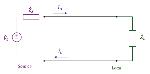
In this idealized circuit the forward current consists only of the differential current ![]() D flowing from the source to the load, while the return current consists only of the differential current
D flowing from the source to the load, while the return current consists only of the differential current ![]() D equal in magnitude and flowing in the opposite direction from the load to the source.
D equal in magnitude and flowing in the opposite direction from the load to the source.
Let’s keep in mind that these are not DC currents. These are high-frequency RF currents that propagate as current (and voltage) waves, and have EM waves associated with them, as shown in Figure 6.
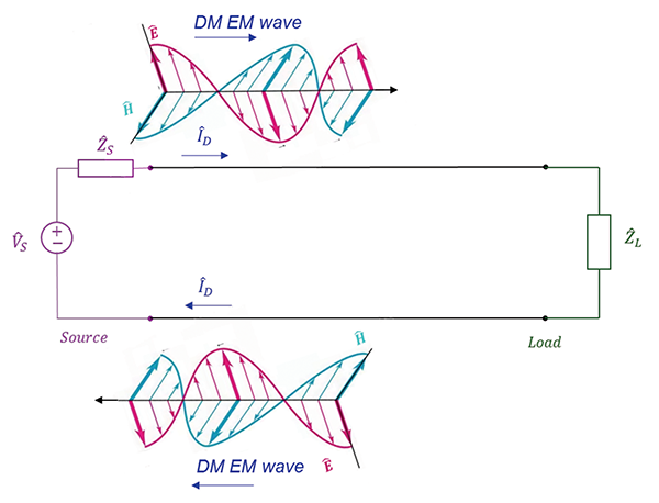
Now consider the scenario where the circuit shown in Figure 6 is in the far-field of another source that generates uniform plane EM waves, as shown in Figure 7.
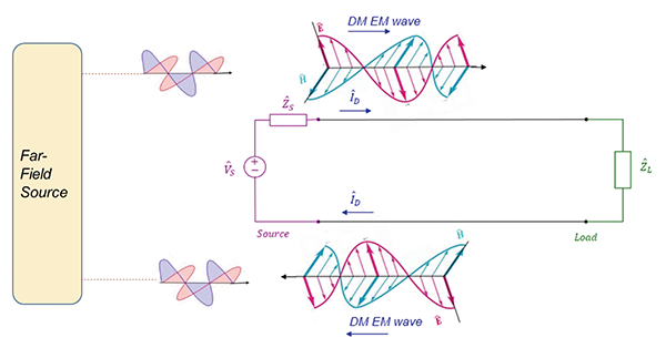
Note that the waves generated by the far-field source propagate in the same direction. When the far-field waves arrive at the original circuit we have a scenario shown in Figure 8.
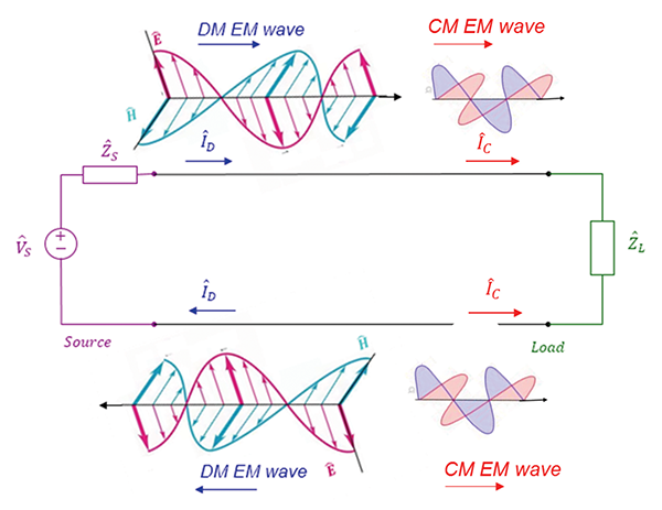
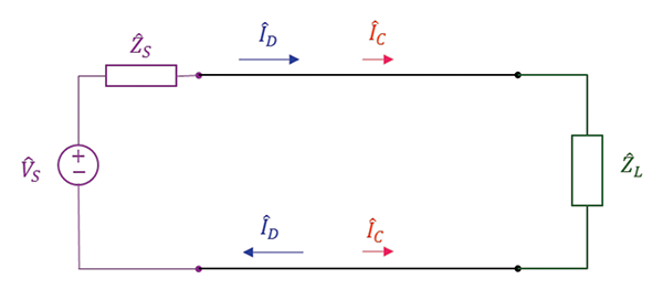
Just like the differential-mode current has a DM wave associated with it, the CM wave has a corresponding CM current, as shown in Figure 8. When drawing electrical circuits, we normally do not show the associated EM waves, and thus a typical DM/CM current circuit is shown simply as the circuit in Figure 9.
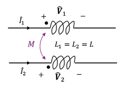
CM Current Suppression Using CM Choke
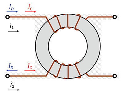
A common-mode choke, shown in Figure 10 consists of a pair of wires carrying currents ![]() 1 and
1 and ![]() 2 wound around a ferromagnetic core.
2 wound around a ferromagnetic core.
As we shall see, the common-mode choke (ideally) blocks the common-mode currents and has no effect on the differential-mode currents.
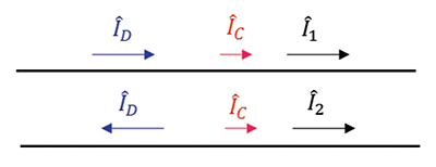
The currents shown in Figure 10 and the total current flowing in each wire, are shown in Figure 11.
Let’s investigate the effect of the choke on the CM and DM mode currents. The circuit model of the choke is shown in Figure 12, where L1 and L2 are the self inductances of each winding and M is the mutual inductance [1, 2].
Using the model in Figure 12 we calculate the impedance of each winding as
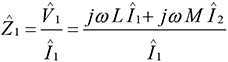 (5a)
(5a)
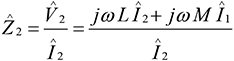 (5b)
(5b)
To determine the effect of the choke on the DM currents let
![]() (6a)
(6a)
![]() (6b)
(6b)
Using Eqs. (6) in Eq. (5a) we get
 (7a)
(7a)
Similarly, using Eqs. (6) in Eq. (5b) we get
 (7b)
(7b)
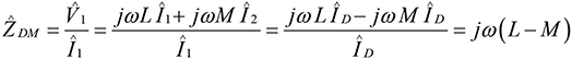
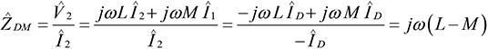
Thus, the impedance seen by the DM current in each winding is
![]() (8)
(8)
In the ideal case, where L = M, we have
![]() (9)
(9)
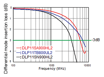
Thus, the ideal CM choke is transparent to the DM currents, i.e., it does not affect them at all over the entire frequency range. Equivalently, the differential-mode insertion loss of an ideal CM choke should be 0 dB over the entire frequency range. Non-ideal, realistic CM chokes exhibit the DM insertion loss similar to the one shown in Figure 13 [3].
Next, let’s determine the effect of the choke on the CM currents. Towards this end let
![]() (10a)
(10a)
 (10b)
(10b)
Using Eqs. (10) in Eq. (5a) we get
 (11a)
(11a)
Similarly, using Eqs. (10) in Eq. (5b) we get
 (11b)
(11b)
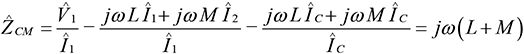
Thus, the impedance seen by the CM current in each winding is
![]() (12)
(12)
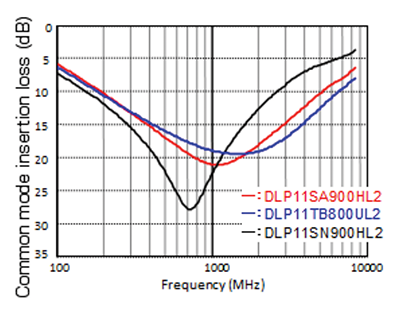
Thus, the CM choke inserts an inductance L + M in each winding, and consequently, it tends to block CM currents. Ideally, this total inductance should be very large over the entire frequency range. Equivalently, the common-mode insertion loss of an ideal CM choke should be very large over the entire frequency range. Non-ideal, realistic CM chokes exhibit the CM insertion loss similar to the one shown in Figure 14 [3].
References
- Clayton R. Paul, Introduction to Electromagnetic Compatibility, Wiley, 2006.
- Bogdan Adamczyk, Foundations of Electromagnetic Compatibility with Practical Applications, Wiley, 2017.
- https://www.murata.com/en-us/products/emc/emifil/selectionguide/highspeed